Data Access
Data scientists know that one of the biggest challenges they face is managing data. By delivering imagery that is sorted and structured ARD reduces the time needed to organize data. It also allows access tools to work in an automatic manner.
ARDCollections have methods that can read (and then also write) windows of data. The software handles finding the intersecting images and reading the pixels for you so you don't have to spend time iterating through image tiles yourself.
Deforestation Example
One of the Maxar ARD sample datasets covers deforestation over time near Rio. Looking at one of the tiles in QGIS revealed this dam creating a pond:
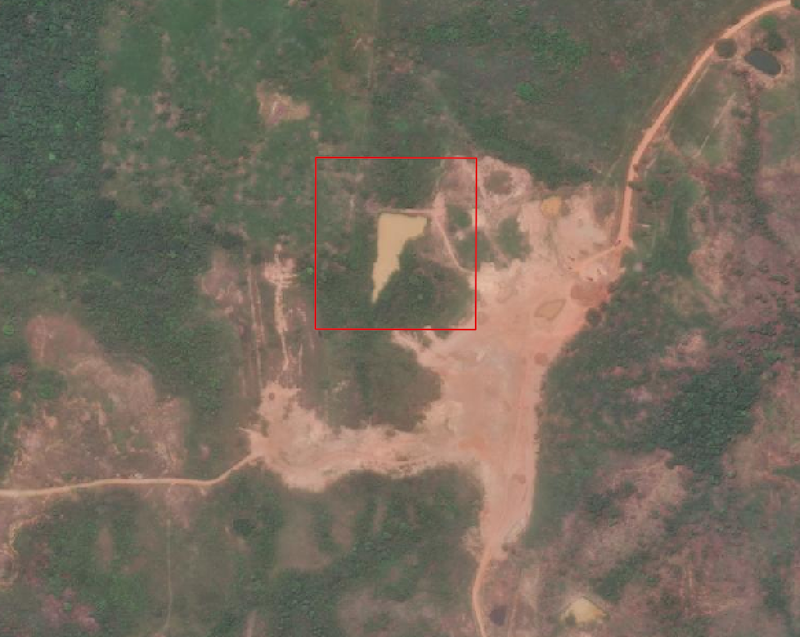
We'd like to leverage ARD to see when this dam first appeared in the ARD tiles.
In QGIS we drew the red AOI and exported it as GeoJSON to use as bounds for our image chips.
First, let's import some libraries:
# ARDCollection to work with data
from max_ard import ARDCollection
# Fiona and shapely to load our AOI geometry from a GeoJSON file
import fiona
# Modules for displaying and writing images
import os
from rasterio.plot import show
import matplotlib.pyplot as plt
%matplotlib inline
To get started, we'll create an ARDCollection of the Rio sample data.
Note: because the sample data is in a public AWS S3 bucket, for a simpler setup we'll pass public=True to disable authentication.
We can see that there are 24 tiles, and they all cover the same ARD Grid tile: z19-300022033202.
collection = ARDCollection('s3://maxar-ard-samples/v4/rio_deforestation', public=True)
collection.tiles
[<ARDTile of 105041000218BB00 at z19-300022033202>,
<ARDTile of 1050410001B2E100 at z19-300022033202>,
<ARDTile of 103001000AC5B000 at z19-300022033202>,
<ARDTile of 103001000CB3FD00 at z19-300022033202>,
<ARDTile of 103001001826FC00 at z19-300022033202>,
<ARDTile of 1050410000818900 at z19-300022033202>,
<ARDTile of 1050410002473100 at z19-300022033202>,
<ARDTile of 10300100253F7900 at z19-300022033202>,
<ARDTile of 1030010026C30800 at z19-300022033202>,
<ARDTile of 10300100296ED400 at z19-300022033202>,
<ARDTile of 10504100105F9E00 at z19-300022033202>,
<ARDTile of 1030010044098C00 at z19-300022033202>,
<ARDTile of 105001000A224100 at z19-300022033202>,
<ARDTile of 105001000A3F3700 at z19-300022033202>,
<ARDTile of 10500100108C6000 at z19-300022033202>,
<ARDTile of 1050010010B6CE00 at z19-300022033202>,
<ARDTile of 105001001583E900 at z19-300022033202>,
<ARDTile of 103001009A654D00 at z19-300022033202>,
<ARDTile of 103001009D8E0A00 at z19-300022033202>,
<ARDTile of 103001009E4FAD00 at z19-300022033202>,
<ARDTile of 105001001BD5A600 at z19-300022033202>,
<ARDTile of 10300100AC6F6800 at z19-300022033202>,
<ARDTile of 10300100ABB61700 at z19-300022033202>,
<ARDTile of 1050010020C7EE00 at z19-300022033202>]
In this case we have selected an AOI that is already in this tile, but what if this collection had tiles all over the globe? How would we know which tiles to open, and how do we read just the window we want?
ARDCollection objects have a method which does this all for you.
(If you run the next cell in a notebook you can read the docstring, but here it is for reference:)
ARDCollection.read_windows(geoms, src_proj=4326)
A generator for reading windows from overlapping tiles in an ARDCollection
Args:
geoms: A Shapely geometry object, or a list of geometries
src_proj: An EPSG identifier parseable by Proj4, default is 4326 (WGS84 Geographic)
Yields:
Tuple of:
- ARDTile of tile
- Shapely polygon representing the bounds of the input geometry
in the tile's UTM coordinate system
- a Reader function:
reader(asset)
Args:
asset(str): asset to read: `visual`, `pan`, or `ms`
Returns:
numpy array of data covered by the returned geometry
Example:
geoms = [...]
for tile, geom, reader in read_windows(geoms):
# can check tile.properties, or fetch tile.clouds
# can check if `geom` intersects with clouds
data = reader('visual')
# shows the docstring in a notebook
?ARDCollection.read_windows
We'll need the AOI geometry from the GeoJSON file, so we'll open the file with fiona. read_windows() can work directly with a Fiona dataset reader so there's no need to open the file and parse out geometries. Note that while we've named this chips, there's only one polygon in this file.
chips = fiona.open('rio-chip.geojson')
read_windows() returns a generator that will yield a tuple of the following for every intersecting ARD tile in the ARDCollection:
- the intersecting ARDTile object
- the input geometry, reprojected to the tile's UTM coordinate system
- a reader function:
reader(<asset name>)
The reader function, when called with a name of the raster asset (visual, pan, or ms), will return a Numpy array of the window covering the bounds of the input geometry.
So in a very simple example, we'll loop through windows with read_windows() and the features read by Fiona. Then we'll use Rasterio's show method to plot the image:
for tile, geom, reader in collection.read_windows(chips):
# reader is a function, so you call it with the asset name
show(reader('visual'))


If you scroll down through the tiles, you'll notice some of them are cut off or even empty of data, and some are covered in clouds.
Since read_chips also returns the projected chip geometry and an ARDTile object, we can do some checks to see if the chip intersects any of the vector ARD masks that are exposed as ARDtile attributes. If they do, we'll skip that tile.
for tile, geom, reader in collection.read_windows(chips):
# skip if the chip geometry intersects any clouds:
if geom.intersects(tile.cloud_mask):
continue
# skip if the chip geometry intersects any nodata:
if geom.intersects(tile.no_data_mask):
continue
show(reader('visual'))
While show() is an easy way to view the images, it would be much nicer to see them in grid labeled by date and without the axes labeled.
Let's create a nicer Matplotlib figure:
# set up a new figure
fig = plt.figure(figsize=(12,24))
# Loop through the windows as before
index = 1
for tile, geom, reader in collection.read_windows(chips):
if geom.intersects(tile.cloud_mask):
continue
if geom.intersects(tile.no_data_mask):
continue
# Create a subplot
ax = fig.add_subplot(6,3,index)
ax.set_axis_off() # turn off the axes
show(reader('visual'), ax=ax, title=tile.date) # add a title using the tile's date
index += 1
# makes a nicer looking plot
plt.tight_layout()

Like read_windows(), there is also a matching write_windows that works in a similar way. Instead of a function you can call to read data, the generator returns a function that can be called to write the data.
writer(asset, path, **kwargs)
Args:
asset(str): asset to read: `visual`, `pan`, or `ms`
path(str): path and name to write the file to.
Kwargs:
driver(str): default is 'GTIFF', but can be 'JPEG' or any other support GDAL driver
Additional keywords are passed to Rasterio's `open` method to create the output file.
Returns:
None
try:
os.mkdir('./chips')
except:
pass
for tile, geom, writer in collection.write_windows(chips):
# filter
if geom.intersects(tile.cloud_mask):
continue
if geom.intersects(tile.no_data_mask):
continue
# generate a name and path for the chip
name = f'./chips/{tile.acq_id}-chip.jpg'
# Call the writer function with the source asset name and the path for the chip.
# Default behavior is to use the GTIFF driver but we'll write JPEGs instead
writer('visual', name, driver='JPEG')
os.listdir('./chips')
['105001000A3F3700-chip.jpg',
'105041000218BB00-chip.jpg',
'103001000AC5B000-chip.jpg.aux.xml',
'103001009A654D00-chip.jpg.aux.xml',
'103001000AC5B000-chip.jpg',
'105001000A3F3700-chip.jpg.aux.xml',
'103001000CB3FD00-chip.jpg.aux.xml',
'10300100AC6F6800-chip.jpg',
'10300100253F7900-chip.jpg',
'103001009D8E0A00-chip.jpg.aux.xml',
'1030010044098C00-chip.jpg',
'103001000CB3FD00-chip.jpg',
'103001009D8E0A00-chip.jpg',
'1050010010B6CE00-chip.jpg.aux.xml',
'105041000218BB00-chip.jpg.aux.xml',
'10300100296ED400-chip.jpg.aux.xml',
'105001000A224100-chip.jpg',
'1050410002473100-chip.jpg',
'10300100ABB61700-chip.jpg',
'103001009A654D00-chip.jpg',
'10300100296ED400-chip.jpg',
'105001001583E900-chip.jpg',
'105001001583E900-chip.jpg.aux.xml',
'105001000A224100-chip.jpg.aux.xml',
'1030010044098C00-chip.jpg.aux.xml',
'10500100108C6000-chip.jpg.aux.xml',
'10500100108C6000-chip.jpg',
'10300100ABB61700-chip.jpg.aux.xml',
'1050010010B6CE00-chip.jpg',
'1050410002473100-chip.jpg.aux.xml',
'103001001826FC00-chip.jpg.aux.xml',
'1050010020C7EE00-chip.jpg.aux.xml',
'10300100253F7900-chip.jpg.aux.xml',
'103001001826FC00-chip.jpg',
'10300100AC6F6800-chip.jpg.aux.xml',
'1050010020C7EE00-chip.jpg']
Putting this all together, a minimalist chipping example that writes chips with incrementally numbered names is:
collection = ARDCollection('path/to/data')
chips = fiona.open('path/to/geojson')
for index, (tile, geom, writer) in enumerate(collection.write_windows(chips)):
name = f'./chips/chip-{index}.tif'
writer('visual', name)
The window functions can handle a single geometry or an iterable of geometries for input. If you need a reference to the original geometry object, you can loop over the geometries outside the generator and feed them individually.
collection = ARDCollection('path/to/data')
chips = fiona.open('path/to/geojson')
for chip in chips:
for index, (tile, geom, writer) in enumerate(collection.write_windows(chip['geometry'])):
name = f'./chips/chip-{chip["properties"]["id"]}-{tile.acq_id}.tif'
writer('visual', name)
Reading outside tiles
Since ARD tiles are gridded, what happens when reading a window that spans across tile boundaries?
read_windows and write_windows can handle a window extending beyond the extent of an ARD tile. In this example over San Francisco we read a window that extends beyond the image apron of the tile on the left.
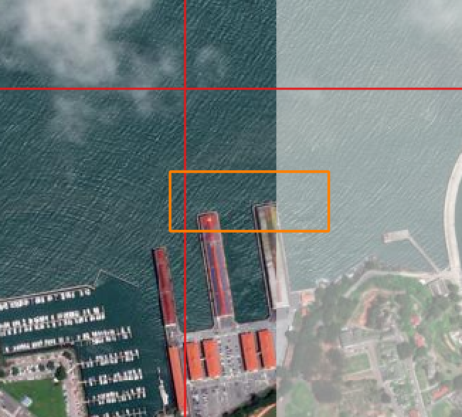
When we plot the windows, we can see that they only contain data and the window has been clipped to the data extents.
collection = ARDCollection('s3://maxar-ard-samples/v4/sample-001', public=True)
collection.tiles
[<ARDTile of 104001002124FA00 at z10-120020223023>,
<ARDTile of 1040010022712A00 at z10-120020223023>,
<ARDTile of 103001005C2E5E00 at z10-120020223023>,
<ARDTile of 1040010022712A00 at z10-120020223032>,
<ARDTile of 103001005C2E5E00 at z10-120020223032>,
<ARDTile of 103001005D31F500 at z10-120020223032>]
chips = fiona.open('outside-sf.geojson')
for tile, geom, reader in collection.read_windows(chips):
# reader is a function, so you call it with the asset name
show(reader('visual'))


Reading across tiles
As shown above, ARD tiles have an apron of pixels that can help read pixels from windows that aren't completely within the ARD grid cell. However, if you have a window that is larger than the overlapped area, a single tile can't fill the whole window.
It is possible to take ARD tiles from the same acquisition and composite them together as a GDAL VRT (Virtual Raster). However the dynamic range of ARD tiles is adjusted per tile so the stack of tiles over a given grid cell look more consistent over time. This means that in certain cases two neighboring tiles might have slightly different dynamic ranges and a seam would be visible. VRTs also have a set stacking order so there is no logic to pick the best pixel source when merging image tiles together.
To address some of these limitations with VRTs, the SDK lets you open a reader on Acquisition objects and read seamless windows from the acquisition's tiles. The component pixels are histogram matched to the source that covers the largest portion of the window to minimize visible seams.
Acquisition.open_acquisition() returns an AcquisitionReader object. The reader object then has a read() method:
AcquisitionReader.read(aoi, asset, src_proj=4326, match=True) -> NDArray
aoi: The AOI to read. This can be almost any geometry object, and if not rectilinear its bounds will be usedasset: The asset to read, such asvisualsrc_proj: Optionally an EPSG code of the AOI's projection (default is 4326)match: An optional argument to enable/disable color matching (default is true)
Like rasterio and the window readers, this method returns a Numpy NDArray.
Note: this function does not support reading across UTM zones at this time.
For example, using the ARDcollection above, we can read a window from each acquisition:
# there are four acquisitions in this collection, two have adjacent tiles
collection.acquisitions
[<Acquisition of 104001002124FA00 [<ARDTile at Z10-120020223023>]>,
<Acquisition of 1040010022712A00 [<ARDTile at Z10-120020223023>, <ARDTile at Z10-120020223032>]>,
<Acquisition of 103001005C2E5E00 [<ARDTile at Z10-120020223023>, <ARDTile at Z10-120020223032>]>,
<Acquisition of 103001005D31F500 [<ARDTile at Z10-120020223032>]>]
for acquisition in collection.acquisitions:
# get a reader at the acquisition level
reader = acquisition.open_acquisition()
# loop through the chips (though there's only one polygon in this example)
for chip in chips:
show(reader.read(chip, 'visual'))

Reading at the acquisition levels returns four windows:
- One that is incomplete because there is only one tile in the acquisition and it doesn't cover the AOI
- Two that are completely filled by loading data from adjacent tiles
- One that is completely filled because the one tile in the acquisition covers the AOI